Hypothesis Testing

Statistical hypothesis testing can be very confusing at first. From its inception, Fisher disagreed with Neyman and Pearson on its use and role in science. Neyman and Pearson argued that they were bringing mathematical rigor to Fisher’s approach, but Fisher considered their framework incompatible with any real day-to-day scientific practice. Unfortunately, no method was ever declared a clear winner, and often hypothesis testing is taught as a hybrid of the two approaches that resulted from confusion by writers of statistical textbooks (as predicted by Fisher) beginning in the 1940s. Furthermore, in the current era where data trumps and nonparametric methods like deep learning are king, many people only get a brief introduction to formal statistics in a data science or machine learning course. It doesn’t help that the professors often don’t need or use hypothesis testing in their daily research any more than their students will in their future employment, and so the subject is quietly brushed under the carpet and quickly forgotten.

Perhaps if we had better statistical education our scientific journals wouldn’t be filled with false research findings. Life does have a tendency to get hectically busy, so no one can be blamed, but I am a firm believer that knowledge acquisition should remain driven by real-world demand and events. With the current COVID-19 global pandemic constantly in the news lately and companies like Pfizer and BioNTech recently announcing a vaccine with 90% efficacy in clinical trials, there doesn’t seem to be a better time than now to learn about hypothesis testing! Not only will this knowledge help you understand and critique the claims being made by researchers and journalists, it will also very likely transfer to other areas of interest to you, whether they be economics, electrical engineering, or particle physics, just to name a few.

What are we testing?

Anyone who has taken a course in statistics or tried learning from reading Wikipedia probably has nightmares filled with endless lists of terms such as

and seemingly insightful diagrams such as

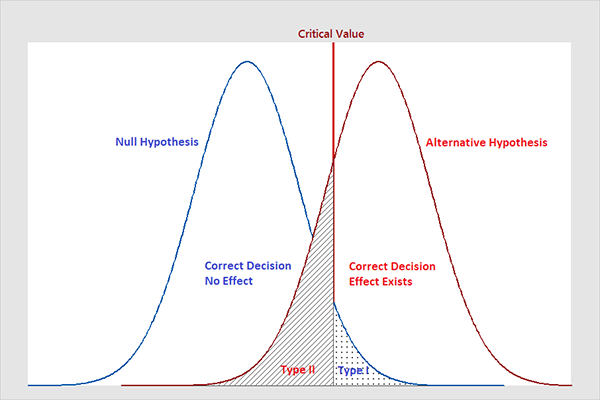
Let’s forget about all of this for now and get back down to the very basics, as Fisher, Pearson, and Neyman did. At the core of any statistical analysis is a probabilistic model, which represents how data is generated. We write $X_i \stackrel{iid}{\sim} f_\theta$, and read “$f_\theta$ is a model for $X$” to mean that the data samples $X_i$ are sampled iid from the probability distribution $f_\theta$.

Given a model and data, there are thus two natural question to ask, depending on whether we know the model to be accurate:

• Anomaly Testing¹ (we trust the model): is this data a representative sample under this model?
• Hypothesis Testing (we trust the data): is this model likely to have generated the data?

Surprisingly, we will see that in many cases, these two seemingly different questions are answered by performing the exact same test! Only the conclusion reached is different. For example, suppose that our model is $X \sim N(0,1)$, that we have a data point $X = -2.3$, and that the test is “reject if $\lvert X \rvert > 1.96$”.

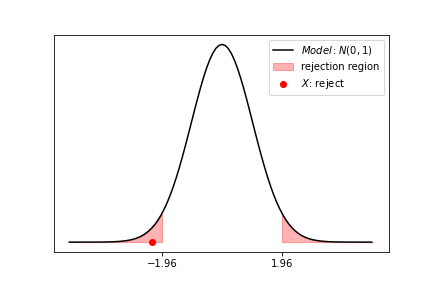
In this case, $X$ fall into the rejection region in red, so we reject! What exactly do we reject? If we know for sure that the model is correct, then we reject $X$ as being anomalous. If instead we know $X$ is a representative sample of the distribution, then we reject the model itself. Perhaps we need to update our model to being $X \sim N(-2,1)$. Before delving into the details of testing, let’s start by putting our Fisherian hat on and contextualizing our statistical inquiry with a more tangible example.

A manufacturing example

Let’s suppose you are the owner of Charlie Chaplin’s factory.

Charlie’s assembly line is manufacturing bolts specified to be 25cm wide. In order to safeguard the solid reputation of your factory, you ask Charlie to reject all anomalously wide bolts, those either too small or too long. After quality controlling a day’s output of bolts, you conclude that their width is well modeled by a normal distribution centered at 25cm with a 0.01cm standard deviation. Arguing that a 0.03cm error off of 25cm is invisible to the naked eye, you decide to reject only those bolts with width outside of [24.97,25.03]. According to the 3-sigma rule, this entails that Charlie will be throwing away 0.3% of the bolts produced, which you deem reasonable.

A year later, Charlie’s end-of-day report mentions having thrown away 3% of that day’s worth of bolts, which represents a lot of money. Is Charlie an incompetent that should be fired, was this just an anomalous day, or does this only mean that the bolt-producing machine needs repair? Perhaps an altogether different explanation is behind this situation? Solving this question requires hypothesis testing knowledge.

Detecting the anomalous bolts was clearly an anomaly detection problem, and deciding which theory best explains Charlie’s lousy day is clearly a hypothesis testing problem. But as we have seen above, these two concepts are really not that different. The “was this just an anomalous day” hypothesis was thrown in the list of theories to highlight their connection!

Formalizing the problem

In order to solve the above question scientifically, we need to first recognize which parts are amenable to statistical analysis. The core issue is whether the machine needs repair or not. Since our statistical model of the machine is $X_i \sim N(25,0.01^2)$, where $X_i$ are the bolts produced, being broken means that either $\mu \neq 25$, or $\sigma \neq 0.01$. In statistical parlance, we write:

\[\begin{align} H_0&: \mu = 25cm, \sigma = 0.01cm \\ H_1&: \mu \neq 25cm, \sigma \neq 0.01cm \end{align}\]

$H_0$ is refered to as the null (default) hypothesis, and $H_1$ as the alternative hypothesis. Our goal is to perform some test to determine which of these is true. In order to simplify our statistical life, we will first assume that that the machine can only break in its $\mu$ parameter. This will turn our test into a simpler test of the mean, which we write:

\[\begin{align} \tag{two-sided alternative} \label{two-sided alternative} H_0&: \mu = 25cm \\ H_1&: \mu \neq 25cm \end{align}\]

This is still just a formalization of our initial scientific/engineering question. Indeed, let’s revisit our three initial hypotheses/theories:

• Is Charlie incompetent? This will be answered indirectly by knowing the state of the machine.
• Was this just an anomalous day? This will be the case if $H_0$ is true.
• Is the machine broken? This will be the case if $H_1$ is true.

Now we need to answer this formal question, and we do so by further translating it into a statistical procedure, a test. Unfortunately, we can’t completely rid ourselves of stochasticity because such is life: machines sometimes break, and sometimes only temporarily; perhaps some old oil was clogging a pipe, but it will melt overnight. One thing we can do, and ought to do though, is to rid our procedure of bias. We cannot use the data collected by Charlie today, because we still haven’t confirmed that he isn’t the reason behind the high rejection rate. What we need to do is to take another worker at random, and have him create 100 bolts the following day. If we have more time, money, and energy to dedicate to this process, we could also require 10 different workers to procedure 1000 bolts each.

Let’s assume for now that we will be producing 100 bolts. Conceptually, our test will consist in measuring the average width of these bolts and making sure that it is not too “anomalous” if those bolts were produced by the null hypothesis distribution. Mathematically, each bolt width $X_i$ is generated from a $N(\mu, 0.01^2)$ distribution. The average bolt width $\bar{X} = \frac{1}{n} \sum X_i$ thus follows a $N(\mu, \frac{0.01^2}{n})$ distribution. Hence, $ \frac{\bar{X} - \mu}{0.01/\sqrt{n}} $ comes from a $N(0,1)$. Using $n=100$ and $\mu_0 = 25$, we find that under the null hypothesis, $ \frac{\bar{X} - 25}{0.001} \sim N(0,1)$, and hence, in 95% of cases, its value will fall between -1.96 and 1.96. In the other 5% of cases, we will declare the machine broken. That’s it, that is our hypothesis testing procedure. Graphically:

In summary, our test is

\[\tag{two-sided test} \label{two-sided test} | \frac{\bar{X} - \mu_0}{\sigma/\sqrt{n}} | > 1.96\]

How powerful is our test?

To recap, we start by measuring the width of 100 bolts, and then form some arbitrary-looking statistic ($ \frac{\bar{X} - \mu}{0.01/\sqrt{n}} $) out of these measurements, and then apply some other seemingly arbitrary cutoff threshold (Z > 1.96) to decide on whether or not to reject the null hypothesis (and declare the machine broken). Why this specific statistic and not some other function of the bolt widths? Could we have used the median instead of the mean? Or the max width obtained? All of these are indeed possible, and would be valid choices. How do we decide which is best then? In order to compare them properly, we now introduce what is called the power of a test. We will see in the next section that our test is indeed the most powerful one.

The power of a test is defined as the probability of correctly rejecting the null hypothesis.

\[\text{Power}: P(\text{reject } H_0 | H_1 \text{is true})\]

Power is a probability, so it is always between 0 and 1. Note that we can easily get power 1 by choosing our test to always reject $H_0$. This would make our test pointless however. In order to prevent this, we also need to balance power with significance, which is the probability of incorrectly rejecting the null hypothesis (you can play with the below widget to get a feeling for their relationship). Significance is also often called type-1 error or false positive.

\[\text{Significance}: P(\text{reject } H_0 | H_0 \text{is true})\]

The commonly accepted methodology for comparing tests is then to set a significance level, typically at 0.05, and then look for the most powerful test among all tests with that significance level.

To make equation writing and diagram drawing easier, we will allow ourselves one further cosmetic simplification to the alternate hypothesis: that the machine can only breaks by becoming looser. That is, $\mu$ can only get bigger, and not smaller:

\[\begin{align} \tag{one-sided alternative} \label{one-sided alternative} H_0&: \mu = 25cm \\ H_1&: \mu > 25cm \end{align}\]

The test also needs to be adapted: \(\tag{one-sided test} \label{one-sided test} \frac{\bar{X} - \mu_0}{\sigma/\sqrt{n}} > 1.64\)

One last very important thing to note, is that the power of a test, unlike the significance of a test, depends on the true value of the parameter in the alternative hypothesis $H_1$. When we write $\mu > 25cm$, we are saying that our test will be valid against any alternative hypothesis. If we knew that everytime the machine breaks, it produces bolts 50cm wide, then it would be very easy to detect it: our test would have great power against this alternative hypothesis! Play with the below widget to get an intuitive feeling for the relationship between $H_1$, significance, and power.

Most Powerful Test: Neyman-Pearson Lemma

In this section we will see that our simple looking test, which compares the mean bolt width to some predefined value, is in fact the most powerful for any given significance level. Note that “the” most powerful test here is really a family of tests. Indeed, for any test, say $\sum x_i > c$, there are an infinite amount of equivalent tests, such as $2\sum x_i > 2c$ and $\log(\sum x_i) > \log c$. Hence, “the” most powerful test is really a family of tests, and we just need to find one among them. Neyman and Pearson proved that the likelihood-ratio test is always among the family of most powerful tests. By simplifying the likelihood-ratio test, we can in many cases recover a much simpler, and more intuitive test.

The LR test, unlike our simple \ref{one-sided test} above, requires specifying an alternative hypothesis. For $H_0: X \sim f_{\theta_0}$ and $H_1: X \sim f_{\theta_1}$, the likelihood-ratio test simply says that $H_0$ is rejected if $\frac{f_{\theta_1(x)}}{f_{\theta_0}(x)} > c$, for some constant $c$ which is set so as to obtain a certain significance level (often 0.05). This however requires knowing the LR distribution, which is sometimes hard to find, and justifies looking for a simplification whose distribution is standard.

For example, using our factory example,

\[\begin{align} H_0&: X \sim N(\mu_0, \sigma^2) \\ H_1&: X \sim N(\mu_1, \sigma^2) \end{align}\]

the likelihood ratio is given by

\[\begin{align} LR = \frac{f_{\theta_1(x)}}{f_{\theta_0}(x)} &= \frac{\frac{1}{\left(2 \pi\sigma^2\right)^{n / 2}} \exp \left(-\frac{\sum\left(x_{i}-\mu_{1}\right)^{2}}{2 \sigma^{2}}\right)}{\frac{1}{\left(2 \pi r^{2}\right)^{1 / 2}} \exp \left(-\frac{\sum\left(x_{i}-\mu_{0}\right)^{2}}{2 \sigma^{2}}\right)} = \exp \left( \frac{2(\mu_1 - \mu_0) \sum x_i + n(\mu_0^2 - \mu_1^2)}{2\sigma^2}\right) \end{align}\]

finding the distribution for this LR seems like an unsurmountable task, but using our \ref{one-sided alternative} assumption, we can simplify as follows

\[\begin{align} \log(LR) &= \frac{2(\mu_1 - \mu_0) \sum x_i + n(\mu_0^2 - \mu_1^2)}{2\sigma^2} > \log c \\ &\stackrel{\mu_1 > \mu_0}{\Longrightarrow} \sum x_i > \underbrace{\frac{2\sigma^2 \log c - n (\mu_0^2 - \mu_1^2)}{2(\mu_1 - \mu_0)}}_{c'} \end{align}\]

One last cosmetic modification will recover our original \ref{one-sided test}

\[\frac{\frac{\sum x_i}{n} - \mu_0}{\sigma/\sqrt{n}} > \underbrace{\frac{c'/n - \mu_0}{\sigma/\sqrt{n}}}_{c''}\]

We have thus shown that our \ref{one-sided test} is in fact equivalent to the likelihood-ratio test, which by the Neyman-Pearson Lemma, is guaranteed to be the most powerful at any fixed significance level.

Summarizing, tests are created by transforming a test sample $X = (X_1,\dots, X_n)$ into a scalar test statistic $T(X)$, which we can then threshold $T(X) > c$ to get a dichotomous answer. The likelihood-ratio test is the most powerful test, but it often leads to test statistics whose distribution we don’t know, and also whose threshold value $c(\theta_0, \theta_1)$ depends on the specific alternative hypothesis. In many cases however, we can simplify the LR to find an equivalent test statistic whose threshold value $c(\theta_0)$ is independent of the alternative hypothesis!

Here is a list of some popular exponential family distributions, their likelihood ratio, as well as its simplication into an equivalent but intuitive test.

Model	Param	LR $\frac{f_{\theta_1(x)}}{f_{\theta_0}(x)}$	Test Statistic $T(X)$	Test
$N(\mu, \sigma^2)$	$\mu$	$\exp\left(\frac{2(\mu_1-\mu_0)\sum x_i + n(\mu_0^2 - \mu_1^2)}{2\sigma^2} \right)$	$\sum X_i | H_0 \sim N(n\mu_0, n\sigma^2)$	$\mu_1 > \mu_0: \sum x_i > c$ $\mu_1 < \mu_0 : \sum x_i < c$
$N(\mu, \sigma^2)$	$\sigma^2$	$(\frac{\sigma_0}{\sigma_1})^n \exp\left( (\frac{1}{2\sigma_0^2}-\frac{1}{2\sigma_1^2}) \sum (x_i-\mu)^2 \right)$	$\sum \frac{(X_i - \mu)^2}{\sigma_0^2} | H_0 \sim \chi_n^2$	$\sigma_1 > \sigma_0 : \sum \frac{(x_i - \mu)^2}{\sigma_0^2} > c$ $\sigma_1 < \sigma_0 : \sum \frac{(x_i - \mu)^2}{\sigma_0^2} < c$
Exp($\lambda$)	$\lambda$	$(\frac{\lambda_1}{\lambda_0})^n \exp \left( -(\lambda_1 - \lambda_0) \sum x_i \right)$	$\sum X_i | H_0 \sim \text{Gamma}(n, \lambda_0)$	$\lambda_1 > \lambda_0 : \sum x_i < c$ $\lambda_1 < \lambda_0 : \sum x_i > c$
Ber($\pi$)	$\pi$	$\left( \frac{\pi_0(1-\pi_1)}{(1-\pi_0)\pi_1}\right)^{\sum X_i} \left(\frac{1-\pi_0}{1-\pi_1}\right)^n$	$\sum X_i | H_0 \sim \text{Bin}(n,\pi_0)$	$\pi_{1}>\pi_{0}: \sum x_i > c$ $\pi_{1}<\pi_{0}: \sum x_i < c $

Bibliography

• The Guinness Brewer Who Revolutionized Statistics
  Gosset was more concerned with whether a result was practically meaningful than whether it was statistically “significant.” He referred to the concept of statistical significance itself as being “nearly valueless.”
• The Difference Between “Significant” and “Not Significant” is not Itself Statistically Significant (Andrew Gelmand and Hal Stern)
  In making a comparison between two treatments, one should look at the statistical significance of the difference rather than the difference between their significance levels.
• The Shadow Price of Power (Cosma Shalizi)
  The likelihood ratio indicates how different the two distributions — the two hypotheses — are at x, the data-point we observed. It makes sense that the outcome of the hypothesis test should depend on this sort of discrepancy between the hypotheses. But why the ratio, rather than, say, the difference q(x)−p(x), or a signed squared difference, etc.? Can we make this intuitive?

Footnotes