A Quick Tour of Applied Koopman Theory

For a continuous-time dynamical system $\dot{x} = F(x)$ on $\mathbb{R}^n$ with flow map $F_t$, the discrete-time Koopman operators are defined as $K_t g = g \circ F_t$, where $g: \mathbb{R}^n \rightarrow \mathbb{R}$. The continuous-time Koopman operator is then defined as $ \lim_{t \rightarrow 0} \frac{K_t g}{t}$.

Without getting caught up in the mathematical details, the central idea of Koopman is to look at the dynamics on observables $g$:

Irrespective of the underlying state-dynamics, the observable-dynamics are linear! This means that their solution is $g_t = e^{Kt} g_0$. Letting $\epsilon(x) = x$ be the identity observable, we see that solving this equation with $g_0=\epsilon$ gives us a way to solve the underlying state-IVP, since given $x_0$,

The main approach to solving the observable-IVP is to find eigenfunctions $\phi_k$ of the continuous-time Koopman operator and their associated eigenvalues $\lambda_k$, such that $K \phi_k = \lambda_k \phi_k$. and writing $\epsilon$ in terms of them: $\epsilon = \sum_k c_k \phi_k$, since then

There are a few different approaches to finding Koopman eigenfunctions:

• Analytical
  • PDE
  • Eigendecomposition of matrix representation of K
  • Fourier Analysis
• Data-Driven
  • Dynamic Mode Decomposition (DMD)
  • Learning Observables

We show these different approaches on a toy model of Steven Brunton to illustrate how they are related¹.

Toy Model

Steven Brunton, in his notes, section 2.3, gives this example system as a starting point for Koopman.

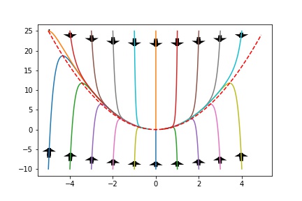
which is interesting because it can be made linear by a finite-dimensional state augmentation. We just need to add $x_3 = x_1^2$, which has dynamics $\dot{x_3} = \frac{dx_1^2}{dt} = 2x_1 \dot{x_1} = 2\mu x_1^2 = 2\mu x_3$, for the system to become:

Analytical Methods

If we have access to equations of motion, a few different methods can find Koopman eigenfunctions exactly.

PDE

Assuming that $\phi$ is an eigenfunction of $K$, eqn $(\ref{koopman-eqn})$ becomes $\frac{d}{dt} \phi = K\phi = \lambda \phi$. Interpreting the dynamics at the level of states, we obtain $\forall x: \frac{d}{dt}\phi(x(t)) = \lambda \phi(x(t))$. Applying the chain rule to the left-hand side, $\frac{d}{dt}\phi(x(t)) = \frac{d \phi}{dx} \frac{dx}{dt} = \nabla_x \phi \cdot \dot{x} = \nabla_x \phi \cdot F(x)$. Putting these together, we obtain the desired PDE

which given dynamics $F(x)$ and an eigenvalue $\lambda$, we can solve to find the eigenvalue $\phi(x)$. Note that this requires knowing/guessing the eigenvalue! As we will see though, these are often easy to guess/derive from the structure of the equation.

We now show how this can be used to find the eigenfunctions of the toy system $\ref{toy-system}$. We start by assuming that $\phi$ is an analytical function, write it using its series expansion $\phi(x) = \sum_{k=0}^\infty \sum_{l=0}^\infty c_{kl} x_1^k x_2^l$, and then play some algebraic gymnastic. Note that this is an oft-used technique for solving differential equations. Now

and so

We’re interested in $\nabla \phi \cdot F(x) = \lambda_{\text{des}} \phi$, which gives

At this stage, we need to start guessing eigenvalues of interest. Due to the simple structure of eqn. \ref{toy-system}, we could guess that $\mu$ and $\lambda$ should be eigenvalues, and we would be right. Finding more eigenvalues is usually easy thanks to the Koopman operator’s eigenvalue lattice structure (see Brunton’s notes section 2.1). Nonetheless, we are already starting to get a feeling for how unwieldy this approach will be for most problems. We will cheat a little here, and save ourselves the tedious algebraic manipulations: we will find the eigenfunctions using another method and only use the above equation to verify that they correct.

The eigenfunctions associated with $\mu$ and $\lambda$ are $\phi_{\mu}(x_1,x_2) = x_1$, and $\phi_{\lambda}(x_1,x_2) = x_2 - bx_1^2$, where $b = \lambda / (\lambda - 2\mu)$. Now we can directly compute

and

Eigendecomposition of matrix representation of K

Let’s start by performing a left eigendecomposition (eigendecomposition of the tranpose) on the matrix in eqn. $\ref{koopman-toy-dynamics}$. The reason for this will and connection to Koopman will be explained shortly.

import sympy as sp
mu = sp.symbols('mu')
lmbda = sp.symbols('lambda')
K = sp.Matrix([[mu, 0, 0],
              [0, lmbda, -lmbda],
              [0, 0, 2*mu]])
print("K:")
sp.pprint(K)
print("Left eigenpairs:")
for eigval,_,eigvec in K.T.eigenvects():
    print(eigval)
    sp.pprint(eigvec[0].T)

Sympy is able to do symbolic matrix decomposition¹:

K:
⎡μ  0   0 ⎤
⎢         ⎥
⎢0  λ  -λ ⎥
⎢         ⎥
⎣0  0  2⋅μ⎦
Left eigenpairs:
lambda
⎡        2⋅μ   ⎤
⎢0  -1 + ───  1⎥
⎣         λ    ⎦
mu
[1  0  0]
2*mu
[0  0  1]

The second and third eigenpairs, associated to $\mu$ were easy to deduce from the diagonal structure of the matrix, or even from the original state-space dynamics, as they correspond to $\frac{d}{dt}x_1 = \mu x_1$ and $\frac{d}{dt}x_1^2 = 2\mu x_1^2$. The first one, associated to $\lambda$, is less trivial. Rescaling it, we obtain $[0,1,-b]$, with $b = \lambda / (\lambda - 2\mu)$, which corresponds to $\frac{d}{dt}(x_2 - bx_1^2) = \lambda (x_2 - bx_1^2)$. This is what we used in the previous section, and is what Brunton finds in his notes. He doesn’t give any justification for this algorithm, instead referring the reader to the Extended Dynamic Mode Decomposition (EDMD) paper. Their proof, however, is matrix-based rather than being operator-based, which is not linear algebra done right, and I find, misses the geometric intuition. We present here an operator-based (basis-free) perspective on this decomposition, in a way similar to how Igor Mezic understands and presents Koopman-related material.

First, let’s look at Brunton’s incomplete Figure 1 of his notes.

The caption reads “Schematic illustrating the Koopman operator for nonlinear dynamical systems”, which leaves the reader wondering how this $K_t$ is related to the actual Koopman operator $K_t$ defined at the beginning of this article: $K_t g = g \circ F_t$. Brunton’s $K_t$ is actually the matrix representation of the Koopman operator in the $g$-basis (we will later write the actual Koopman operator as $U_t$ to keep them separate). But there still seems to be questions left to answer, such as why we needed to take left eigenvectors of $K_t$. Brunton probably opted to hide some of the details to be able to reach a broader and more applied audience. I personally think he oversimplified it too much, which will at at some point result in technical debt needing to be repayed in the form of headaches when trying to understand Igor Mezic’s original papers. That’s certainly what happened to me, and now I get a little annoyed evertime I read a paper calling “nonlinear mapping + least-squares regression” “Koopman”.

The real diagram making the connection between Brunton’s matrix and the real Koopman operator is more involved, but I believe is well worth the effort understanding. We drop the $t$ subscripts for ease of reading, but have to remember that all operators used in this section are the discrete-time versions.

The bottom two rows of the diagram are equivalent to Brunton’s diagram The top part of the diagram is pretty crowded, so we interpret it row-by-row, starting observables, which play a key-role in Koopman theory.

Observables: Observables are, as usual, scalar mappings $g: \mathbb{R}^n \rightarrow \mathbb{R}$ defined on the state-space, and $F$ stands for any class of functions, typically $F=\mathrm{C}^\infty(\mathbb{R}^n)$. The Koopman operator moves these forward in time $g \mapsto Ug$. We use the letter $U$ to refer to the operator itself, leaving the letter $K$ to stand for its representation in different bases, as Igor Mezic does.

Observable coefficients: When we choose a basis for $F$, say \(\Phi = (\phi_k)_{k=1}^\infty\), then we can write both observables and the Koopman operator in this basis. For example, if $g = \sum_k a_k \phi_k$, then we can let \(a=(a_k)_{k=1}^\infty\) stand for $g$, writing $\lbrack g \rbrack_\Phi = a$. This is similar to how in linear algebra, the vector $[v_1,v_2,v_3]$ really stands for \(v=v_1e_1+v_2e_2 + v_3e_3\). We also let $K^T$ be the representation of the Koopman operator $U$ in the basis $\Phi$. That is, if $g_2 = Ug_1$, \([g_1]_\Phi = a_1\), and $[g_2]_\Phi = a_2$, then \(a_2 = [g_2]_\Phi = [Ug_1]_\Phi\) and we define $K^T$ such that \(\lbrack Ug_1 \rbrack_\Phi = K^T a_1\). This is exactly what the top-square of the above commutative diagram is representing: it defines $K$ by forcing both paths from the top-left \((\mathbb{R}^d, \Phi)\) to the bottom-right $F$ to be equivalent for all \(a \in \mathbb{R}^d\). That is, $K$ is defined by being the unique set of coefficients such that

which is just another way of saying $ \left\lbrack U(\sum_d a_d \cdot \phi_d) \right\rbrack_\Phi = K^Ta$.

Using the tranpose might seem arbitrary, and it is! We define it this way so that the bottom part of the diagram matches with that of Brunton. Otherwise, his $K$ would be our $K^T$.

Observations: Observations connect the world of Koopman and observables to the original state-space. An observation $y$ is obtained by evaluating an observable $g$ (or $\phi$!) at a given state $x$: $y = g(x)$. Note that this simultaneously explains both mappings to the observations space $\mathbb{R}^d$: $x_0 \mapsto g(x_0)$ and $g \mapsto g(x_0)$. One of them waits for an observable, while the other waits for a state.

Transpose: The last bit of notation that is worth explaining is the relationship between $K^T$, which evolves observable coefficients (and is hence the matrix representation of the Koopman operator), and $K$, which evolves observations. A priori, there seems to be none, but the fact that they are transposes forces us to find one.

We often write coefficient vectors as row vectors.

This is a slight abuse of notation since we are putting functions $\phi_d$ inside a vector, but it will be well worth once we get passed the original frown. Indeed, it gives a very vivid visual way to remember the relationship between $U$, $K$, and $K^T$!

The strength of this representation is immediately apparent, as we can view $K$ either as right-multiplying $a^T$ ($a^TK \equiv (K^Ta)^T$) or as left-multiplying $\Phi$. Now evaluating $\Phi$ at $x_0$ results in Brunton’s $K_t$ operator from his diagram: $\lbrack Ug \rbrack (x_0) = a^T K g(x_0)$. In short, $K$ moves observations forward in time, whereas $K^T$ moves coefficients forward in time.

Fourier Analysis

The toy example that we are considering in this post is simple enough for simple methods to work. This is not always the case however, and in the more general cases, a Generalized Laplace Analysis might be necessary. We refer the reader to section B.1 of Applied Koopmanism.

Data-Driven Methods

Sometimes we don’t have access to the dynamics’ governing equations. In this case, we can’t derive the Koopman matrix by hand, as we did in eqn. $\ref{koopman-toy-dynamics}$. Instead, we need to learn it from data. Most of the data-driven methods for identifying Koopman eigenfunctions amount to three simple steps:

• Choosing/Learning a dictionary of observable functions
• Performing system identification to identify the Koopman matrix
• Performing an eigendecomposition of this matrix, as we did above

Dynamic Mode Decomposition (DMD)

The DMD algorithm was originally developed by Peter Schmid in 2008 as an algorithm for analyzing fluid flows. A quick look at its wikipedia page is enough to be convinced of its impact, and to be overwhelmed at the multitude of related algorithms. One shouldn’t be scared though, DMD is really nothing more than learning the “Koopman” matrix, and finding its principal eigenvectors. Most of the concerns in DMD related paper are not of much importance to people in the robotics/control community: DMD was originally developed for fluid flow analysis which deals with huge state-space and few datapoints, whereas we have to deal with the opposite case of relatively low-dimensional state spaces (we almost always assume rigid bodies) and large amounts of data (thanks to our simulators). We will thus not get into the details of dimensionality reduction that DMD goes through, as Steven Brunton has already published a short youtube playlist on the subject.

We will simply show that we can recover the exact subspace and dynamics that we derived analytically in eqn. $\ref{koopman-toy-dynamics}$. The code¹ below uses

• A dictionary of observables consisting of polynomial combination of state variables
• A simple least square regression to identify the dynamics on this dictionary of observables
• A basic numpy eigendecomposition to identify the left eigenpairs

import numpy as np
from scipy import linalg, integrate
from scipy.integrate import solve_ivp
from scipy.linalg import logm
from matplotlib import pyplot as plt
from sklearn.preprocessing import PolynomialFeatures
import itertools
import sympy as sp
np.set_printoptions(suppress=True, precision=3, linewidth=np.inf)

class PolyLiftedSpace():
    """Class for lifting state-space with polynomial terms.
    Eg. if n_state=2 and poly_deg=2, then state-space transformation is
    (x,y) -> (x,y,x^2,y^2,xy)"""
    def __init__(self, n_states, poly_deg):
        self.n_states = n_states
        self.poly_deg = poly_deg
        self.poly = PolynomialFeatures(poly_deg, include_bias=False)
        
    def lift(self, X):
        return self.poly.fit_transform(X.T).T

def koopman_operator_lsq(X, X_prime,lifted_space):
    """ Returns the Koopman operator calculated from lifted trajectories resulting from applying
    lifted_space to X and X_prime."""
    Psi = lifted_space.lift(X)
    Psi_prime = lifted_space.lift(X_prime)
    K = linalg.lstsq(Psi.T, Psi_prime.T)[0].T
    return K

# Collecting trajectories for sysid
def run_random_episode_with_init(x0, model, t_range, t_step):
    """ Returns a solution to the IVP x'=model.f(x), with initial value x0."""
    t_eval = np.arange(*t_range, t_step)
    sol = solve_ivp(model.f, t_range, x0, t_eval=t_eval)
    if not sol.success:
        raise RuntimeError(sol.message)
    X = sol.y[:, :-1]
    X_prime = sol.y[:, 1:]

    return X, X_prime

def run_random_episode(x_low, x_high, model, t_range, t_step):
    x0 = np.random.uniform(x_low, x_high, x_low.shape)
    return run_random_episode_with_init(x0, model, t_range, t_step)

def run_random_episodes(num_episodes, x_low, x_high, model, t_range, t_step):
    X, X_p = run_random_episode(x_low, x_high, model, t_range, t_step)

    for i in range(num_episodes - 1):
        X_new, X_p_new = run_random_episode(x_low, x_high, model, t_range, t_step)
        X = np.concatenate((X, X_new), axis=1)
        X_p = np.concatenate((X_p, X_p_new), axis=1)
    
    return X, X_p

mu = -0.05
lmbda = -1
poly_deg = 2 # you can increase this, it still identifies the exact matrix!

t_range = (0, 10)
t_step = 1e-3
x_low = np.array([-10,-100])
x_high = -x_low
num_episodes = 100

sys = BruntonExample(mu=mu, lmbda=lmbda)
X, X_p = run_random_episodes(num_episodes, x_low, x_high, sys, t_range, t_step)

lls = PolyLiftedSpace(n_states=2, poly_deg=poly_deg)
K_dt = koopman_operator_lsq(X, X_p, lls)
K = logm(K_dt)/t_step # continuous-time Koopman
print(K)

[[ -0.05    0.      0.     -0.     -0.   ]
 [ -0.     -1.      1.      0.      0.   ]
 [  0.      0.     -0.1    -0.     -0.   ]
 [ 24.252  -0.195   0.205  -0.586   0.003]
 [-13.925  48.963   3.632   0.635  -1.159]]

The top-left $3\times 3$ matrix is exactly the matrix in eqn. $\ref{koopman-toy-dynamics}$ for the chosen values $\mu=-0.05$ and $\lambda = -1$. You can try changing these and augmenting the max polynomial degree, it is surprising how robust it is!

Learning Observables

Although DMD and related algorithms start from a fixed dictionary of observable functions, the performance of the algorithm will largely depend on this choice of dictionary. As we say, polynomial, fourier, and kernels are often used, hoping one of them will perform well. Another method is to instead learn this dictionary, jointly optimizing for $g$ and $K$. Many different function approximation methods have already been tested, including sparse regression, gaussian processes, and deep learning. We leave the interested reader to deep dive into his/her method of choice.